A January Summary for 2015 Hyperversity

I assume everybody has something for which they care dearly.  The loss of our technologically advanced culture would ruin that thing in every case I can think of.  Sustaining the developed world should be a top priority for everybody.

If what I have to say is understood by a sufficient number of people there is every hope that we shall endure. 

But today the developed world is in a demographic crisis, unable to produce enough babies for survival in the long term.  In the short term things may get worse faster.  The weight of the evidence is that failing to marry kin sufficiently often will destroy a population.  It is obvious that we once married cousins of intermediate consanguinity and now marry cousins of very remote kinship, or as we say “unrelated,” although that is impossible; we then had babies in ample numbers and now do not.  The effect appears to accumulate over generations.  We may be near the end.

If the babies stop coming, all is lost.

Before introducing evidence, let me lay some groundwork. 

I shall be using the word “system” in a very specific way.  For our purposes I define it as, “A physical object through which energy flows with some effect occurring as a consequence.”  For instance a household hammer is a system in this sense.  Kinetic energy is put into the hammer by means of the wielders’ arm; the hammer strikes, and a nail is driven.  Nothing endures forever, so if there are to be systems in the future they must be replaced.  If people make the system we call it a “device.”  If the system replaces itself we say it is “alive.”  Technology may change that, but for now the distinction is good enough.

There are two styles a system may employ in replication: replication can be extremely faithful, as it is for many microorganisms, or there can be reproduction with substantial variability, as with humans.  Microorganisms will not concern us here.  Indeed complex organisms can reproduce with great fidelity; dandelions seem go without sex between two plants without any great loss of viability.  Again, we shall neglect them.

Given that any environment must be finite, those organisms that reproduce with variation must ultimately compete.  There will be winners and loseres in such competition.  Success must depend in part on the inherited variability.  Therefore there must inevitably be selection so that the inheritable characteristics of any population of living things may change over time.

Any complex system can be destroyed by a simpler system, as a fine watch may be destroyed by a hammer.  So complex organisms must be vulnerable to diseases caused by simpler organisms; we get sick.  Were we all identical, than a disease fine tuned to our inherited makeup could wipe us out.  The advantage of defending against this by maintaining some variability is a great, if not the only, advantage of variable reproduction.  (Divided We Stand ECONOMIST vol. 411 no. 8888 May 24, 2014 page 74)

The way we maintain our variability is through sexual reproduction.  We have inheritable pieces of information (that will be used in the creation and maintenance of our bodies) called “genes” that are hooked together in chains called “chromosomes.”  This is oversimplified, but sufficient for now.  The chromosomes occur within the nuclei of the cells of which we are made; each kind of chromosome exists as a pair.  We will neglect sex chromosomes and now only consider the “autosomes,” the others, each chromosome of each pair having a very similar structure but differing in detail.  The differences in those details comprise a great deal of our inheritable variation.  Within a pair an individual inherits one chromosome from one parent and one from the other.  The individual will pass one or the other of its chromosomes to each offspring. 

Selection is a competition.  This is particularly true when a new ecological niche appears.  Some living form that can exploit the niche can, through selection, optimize its ability to exploit that niche and exclude others.  A species is a population that can interbreed and have fertile offspring.  Any members of a species that mates with a different species cannot have offspring that are fertile over many generations.  When a species divides to form two new species, the event is called speciation.  So if selection is a competition, so is speciation.

Let me formalize it thus:
Consider a settled environment containing a species “A” exploiting niche “a,” and species B exploiting niche “b.”  With regards to these niches we do not expect a new speciation event.  A new speciation must await a new niche.  (Arne O. Moores Supply and Demand, NATURE vol. 509 no. 7499 May 8, 2014 page 171 and Trevor Price et al. Niche Filling Slows the Diversification of Himalayan Songbirds page 222 in the same issue.)   So our system will remain stable with Aa and Bb. 

Now a new niche “c” arises.  To a degree both A and B are able to exploit it.  The system is now Aa, Ac, Bb and Bc.  But selection promoting Ac will change A so that it is less efficient at strategy Aa.  It is in danger of being replaced.  Some species C comes from somewhere with the strategy Ca; it is no longer in contact with its population of origin so it can optimize itself for niche a.  Our system is now Ca, Aa, Ac, Bb and Bc.  C can optimize for Ca, but A cannot because it is also “trying” to optimize for Ac.  So A is driven out of a.  So the system will be Ca, Ac, Bb and Bc.   If niche c turns out to be temporary, Ac is lost, Bc is lost and we have Ca and Bb. 

A has been lost altogether even though its niche never changed.  The same threat applies to B. 

Now suppose B can undergo speciation into B1 and B2.  Now B1 continues to exploit b and B2 can exploit c and the system is Aa, Ac, B1b and B2c.  Ac disappears because B2 can outcompete A for niche c, and the new pattern is Aa, B1b and B2c A.  If the new niche closes, B1 is unharmed.  Even if one of the old niches closes, B goes on.  Clearly rapid speciation is an advantage to B.  If it moves quickly to speciation, it can seize the opportunity c from A and C is no threat. 

This contrasts with the only sentence in Darwin’s Origin of Species that was actually about the origin of species (in the version I read).  “As for the origin of species it is happenstance as hybrid infertility never did any species any good.”  Alfred Russel Wallace did understand the principle.  Darwin, because he was rich and could publish his own book before Wallace could publish, got the fame and the truth was lost from view for a time.  Yes, speciation does benefit a species.  Speciation is a race just as selection is a race. 

I used to have two lines of evidence – the speciation of Bactrian camels into Bactrian and dromedary and the speciation of mice in the different valleys in the Canary Islands – that suggested that speciation in mammals occurs after about two thousand generations of separation.  However more recently the word seems to be that there had long been wild dromedaries in Africa; they are not simply the descendants of domesticated Bactrians.  Also there has been found evidence that there were mice in the Canary Islands long before the time of Columbus.  So I must abandon that argument.  I’m not at all sure of it any longer.  I shall assume for now that the rule of two thousand generations to speciation holds, but you may use whatever number you think proper; the logic remains unchanged. 

This rapid speciation confers a benefit, but it comes at a cost.
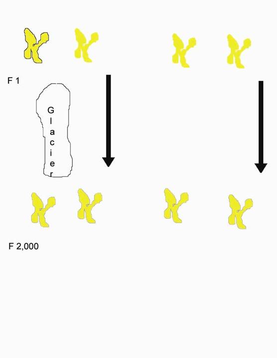
Consider a valley with 1,000 animals, say mice.  One mouse has a particular normal chromosome.
 
It replicates and the two copies wind up in two offspring.  These are as alike as two chromosomes can get to be.

 
One mouse scurries across the valley; a glacier splits the valley in two.  The glacier remains for two thousand mouse generations.  The F2,000  mouse (That is to say a mouse two thousand generations later) from the far side of the valley returns and mates with an F2,000 mouse from the near side.  But they cannot have normal fertile offspring.  There has been speciation.   
Now, instead of a glacier, the mice mate at random throughout the valley, the population being constant at 1,000.  Since there are 2,000 copies of the chromosome it takes on average 2,000 generations before one the F2,000 of the original chromosomes finds itself in the same individual with another F2,000 of the chromosome.  They are as different as if they had been separated for as long by the glacier.  The offspring are not fertile.  Since this is true of every part of every chromosome in every mouse, the population dies.

So the time to speciation has constraints on both sides.  Undergo speciation too slowly and be outpaced by more nimble species as niches open and close.  Undergo speciation too quickly and lose all but the smallest and least successful populations.  What happens must be a compromise.
One might be forgiven for saying that people see the big picture but fail to consider the long view.  Nature takes, as it were, the long view but has no way to deal with the big picture.  If a population that reaches 1,000 is doomed so nature is under great pressure able to select for some robust mechanism that can correct things but cannot do what traditional societies do regularly and say in effect, “There are too many of us in this social pool.  You go over there and we’ll go over here.  And by the way, any stranger that wanders by gets it in the neck so don’t forget that you are now honorary strangers.”  Nature can’t walk around and do a census. 
Nature must work on the small scale, selecting for a mechanism that deals with individuals and mating pairs.  The mechanism must somehow assess the size of the mating pool and make an adjustment, presumably reducing fertility when the pool gets too large.  If there is another way to do it, it is beyond my imagination.  The best evidence must be a demonstration of the fertility of a population changing with population size.  There is a study done by a team led by Richard Sibly.  They looked at over a thousand serial field counts of wild animals and regularly found this relationship:
 

On the Regulation of Populations of Mammals, Birds, Fish and Insects, Richard M. Sibly, Daniel Barker, Michael C. Denham, Jim Hope and Mark Pagel SCIENCE vol. 309 July 22, 2005 page 609
This is presented as a typical species.  The estimated number in the population is on the horizontal axis while the population growth rate is on the vertical.  By the time the population reaches 1,000 the growth rate is negative, and sure enough growth rate falls as population rises.  This happens without respect to limited environmental resources, as that would yield a curve turning the opposite direction. 
A different study was done of captive mice.  A large cage with plenty of room, food and bedding material was prepared.  Four male and four female mice were introduced.  The mice were counted regularly.  This was the result:
 

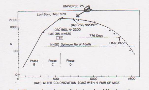
History of population of mice in a closed Utopian universe.  Solid line is actual counts.  Broken line after about 700 days represents an estimate of numbers on the basis of observed mortality.  Points after Day 1000 are slightly lower than projected due to removal of about 150 mice for other studies.  A final point was added to the graph for Day 1471 when the population had decreased to 100. At final editing of this paper on November 13, 1972 (Day 1588) the inexorable decline brought the population to 27 (23females and 4 males, the youngest of which exceeded 987 days of age)
John Calhoun Death Squared: The Explosive Growth and Demise of a Mouse Population Proceedings of the Royal Society of Medicine vol. 66, January 1973 page 80 (The crude arrow is mine.  I initially thought that their estimates might have introduced an error, but on further review and reflection I think they are probably good.)
The population grows exponentially for a time, then grows more slowly.  The last live birth occurs on day 600, at which time all births cease and the population slowly dies out.  (Calhoun himself thought the problem was excessive social contact.  In 1973 there was no text messaging.  As it turns out, people can handle a lot of social contact.)
Obviously this is an effect that nature will not tolerate forever; neither an intelligent designer nor a really stupid designer would either, for that matter.  It is readily observable that most species have more than a thousand members.  So a preventive mechanism must be in place.  It must hold any local population to less than 1,000.  Since if you could go back ten generations with no cousin marriages at all you would have 1,024 ancestors in that generation, the mechanism must require a couple to share a number of ancestors over the previous 10 generations.  Otherwise there will be an eventual population crash as we observe in the mice. 
That is why the mechanism or mechanisms developed.  There is enormous selective pressure in the long run that favors it or them. 
We have already looked at data that demonstrate the mechanism in action.  These two studies are very robust.  Observations were made by skilled professionals in real time with unambiguous meaning.  Certainly studies can be challenged, as can the suggestions from the dromedary and Canary Islands mouse studies. However those studies were attempts to determine what happened in the distant past.  That renders them more vulnerable.  Later we will be looking at some old data also, but the point is already inescapable.  A mechanism or more than one limits fertility when the local breeding population gets large.

Here is data recording plagues of wild mice in Australia and New Zealand.  During a mouse plague the mice increase dramatically in number.  Then the population crashes.  There are mouse counting stations that keep track of this.  The data are accumulated from a few such stations.

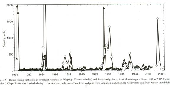
Information from The Mouse in Biomedical Research second edition Volume 1 History, Wild Mice and Genetics, chapter 3 “The Secret World of Wild Mice” section VI Population Dynamics part C. Population Eruptions (Mouse Plagues in Australia; population eruptions in New Zealand) Grant R. Singleton and Charles J. Krebs editors James G. Fox, Muriel T Davisson, Fred W. Quimby, Stephen  W. Barhold, Chritian E. Newcomer and Abigail L. Smith Elsever Burlington 2007 page 39.  The caption reads: House mouse outbreaks in southeast Australia at Walpeup, Victoria (Circles) and Roseworthy, South Australia (Triangles) from 1980 to 2002. Densities exceeded 2,000 per ha (hectare) for short periods during the most severe outbreaks.  Data from Walpeup from Singleton, unpublished; Roseworthy data from Mutze, unpublished.) 

The plagues tend to follow droughts.  We would expect that.  A severe population reduction should reduce all the local mouse populations and make rapid subsequent population growth possible. 

In five of the plagues there is a single very high spike lasting something like a year.  This is not so long as the 600 days to last live birth in the Calhoun study, but is quite consistent with the something over 300 days until the end of the initial exponential growth in the Calhoun study.  We need but accept Calhoun’s assurance that his cage was indeed safer than the wild and the time course is quite compatible.  There are also three plagues that follow a different course.  The peak is lower and there is a second peak that is a bit larger than the first.  We shall return to this pattern presently. 

Here is a collection of data than I am not quite sure how to fit in.  3,000 species across a variety of taxa were studied. Although they reckoned that real population sizes varied over several orders of magnitude, overall they found little (factor of about 10 and simpler seeming forms with larger populations) variation in nuclear DNA over multiple taxa (bottom line), and none at all in mitochondrial DNA (upper line).  They suggest multiple selective sweeps. 

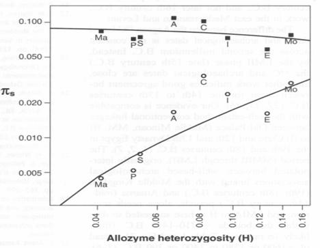
Population Size Does Not Influence Mitochondrial Genetic Diversity in Animals.  Eris Bazin, Sylvain Glémin, Nicolas Galtier SCIENCE VOL: 312 570 28 APRIL 2006.

I agree with the notion of sweeps of population loss.  But I’m not so sure the sweeps are selective in the ordinary sense.  I suspect that if you could envision the different mating pools you would see local populations undergoing rapid growth and then collapse all the time, just as you see in the mouse plagues.  As we radiologists often say, “Consistent with but not diagnostic of” the diagnosis. 

Before leaving animals for a time, there was a study done in which they were establishing a population of black footed ferrets in the wild.  For years they would release ferrets (indicated by the vertical black bars in the graph) and count the animals. 

The last release was in 1994.  They continued the counts until 1997 and then gave up.  The number was falling with no prospect for a viable population.  But when they checked again in 2000 there were ferrets again.  They released no more but followed with counts only missing one year until 2006.  What they have is roughly exponential growth.  The best fit for exponential growth is the red line. 

Now that we know that explosive growth is possible from a small rather homogeneous population, we can see what was going on.  They were releasing too many ferrets and probably not very kin ferrets.  Once they gave up the population was able to decline and increase its consanguinity. This took at least three years, during which there was no growth.  Then when the population was sufficiently homogeneous growth was very rapid.  But the growth was not exactly exponential.  It was below exponential, then above, then below again.  We will return to this observation when we consider humans and when we consider a computer model. 

Notice by the way that this study, which was not included in the Sibly paper because it was still going on, would not have matched his pattern.  It still follows the law his pattern demonstrates of course.  And notice that the count did not exceed 200.  The study was halted because by the time the population had reached such a size ferrets were moving out and establishing new colonies.  They were subdividing their population long before it rose to the toxic heights that Calhoun’s mice and the plague mice reached. 

Of course it is of paramount interest whether this biological mechanism so obvious in animals is effective in humans.  Is a human reproductive rate a matter of “choice” or is it a matter of consanguinity as it is in animals? 
For a quick overview we will look at UN data.  Here is a graph of the world’s birth rate over the past 50 years.  It is a few years old, downloaded August, 2008, but in general things cannot be much different. 

The vertical axis is the average number of children born per woman.  The horizontal axis gives the dates of the surveys. The numbers are broken down into rich world, middle world and poor world.  Except for children born in the past few years everybody under 50 is in one of these columns; this is ALL THE JELLY BEANS, the entire future of humanity since those over 50 don’t add much to the population.  Birth rates are obviously different in different places, and the lines move up and down.  Some people may think there is a significant genetic difference between populations.  Jefferson wrote, “All men (persons) are created equal.”  That may not be the last word, but it is a good place to start.  We are going to see objective evidence that it is so.  What we’ll do now is follow the yellow columns down until they overlap the red columns then jump back to a red column of the same height and follow the red columns until they overlap the blue columns then jump back to a blue column of the same height and follow the blue columns until the end.  Here’s what we get:

It’s all one single curve. You can’t even tell where the cut and pastes happened.  On this one Jefferson was right.  We are all just alike: we are only at different places along the same line.  Notice that the final column levels off and even edges upward slightly.  And in fact lots of rich countries have had an increase in their birth rate, not enough to recover, but some.  When the experts look at this they say or have recently said, “The population will reach a maximum of about 10 billion in about 2050 and then it will stabilize.”  Cool.  And that prediction is based on the assumption that women in the future will have exactly the same number of children at each age as they do now.  But that is obviously wrong.  If it were generally true, the line would have to be straight horizontal.  Demographically speaking, we are all on the same line, just at different places along it.  We are all going to the same place, and from the evidence at hand that place is unsustainably low birth rates for the foreseeable future.  Later we will have to amend this prediction.  For right now, the question is whether fertility is depressed for the same reason as it is in animals, or is the biology of humans that different from other animals?
We may get a clue by comparing the maximum growth rate with that of the black footed ferrets.  Remember growth was below exponential, then above, then below.  We now look at the actual growth rate of the poorest part of the world (which has the highest birth rate) during the time of most rapid growth. 

Offspring per woman in least developed part of the world between about 50 and 75 years ago.

It is the same pattern.  Growth is high, but accelerates before it decelerates, just like the ferrets.  The effect is biological.  Dismiss “choice” from consideration.  We shall return to this again when we discuss mechanisms.

What has been demonstrated is that, so far as we can see from the graphs, which of course may conceal small or very localized differences, the whole population of the world is on a course that will ultimately lead to inadequate fertility.  And there is a hint that the biological mechanism is similar to something about animals.  So what could the precipitating cause be?  There must be something new under the sun.  If this biological process had been in action for all the thousands of generations of humans, obviously we would all have vanished long ago.  So what is different from anything that has gone before?  Obviously it is our splendid technology.  The world has never seen human control over things the likes of this before.  And what could the key element of our technology be?  It seems to me to be that we can get around more easily than ever.  Other things like more food and possibly pollutants could be considered.  But for every other species, it seems that providing food produces population expansion.  The birth rate has been below replacement in the developed world for thirty years.  If diet is the cause, then something very strange is going on.  As far as pollutants, indeed it is possible that our advanced technology has released something chemical that is doing us harm, but people are looking for a culprit and have come up empty handed. 

So the first guess must be it is ease of transportation.  People marry within a bigger social pool than we did only a few generations ago.  The Sibly paper quoted earlier showing the relationship between population size and population growth rate in animals predicts negative growth, and we have it.  That in turn implies that a larger mating pool – which is inversely proportional to average kinship between pairs – means lower fertility.  Lower kinship: lower fertility.

Here is a data set from the genealogies of Iceland.  They chose couples at random, went back ten generations, counted shared ancestors and from that calculated kinship.  The result is not exactly the same as our definition of cousins in English.  If a couple shares a great grand parent, they are second cousins in standard usage but might be closer in their formulation if there are other sources of kinship.  There might be another shared great grand parent. 

With this warning, here is the relationship they found between kinship and fertility.


An Association between Kinship and Fertility of Human Couples Agnar Helgason et al. SCIENCE vol. 329 no. 5864 February 8, 2008 page 813 – 816  The vertical line is number of children “normalized.”  The horizontal line is kinship. 
It is the same curve as Sibly found in animals, except there tends to be a leveling off when one gets below “third cousin or closer.”  “Third cousin” would be half way between “third cousin or closer” and “fourth cousin or closer.”  So they have slightly soft-pedaled the message. 
Look at the exquisite precision.  Those error bars represent two standard deviations.  The data have been “normalized,” which is to say that the actual number of children is compared with the national average for that generation.  So if you know how many children a couple had, and what the Iceland average was for that generation, you tell that they are, for instance, fifth cousins rather than fourth or sixth cousins and be right ninety percent of the time.  You will know their kinship, calculated over the past ten generations, far more accurately than they probably know themselves.  At least this would be the case if there were fractional children.  In real life I’m not so sure. 
They then went on, gratifyingly, to look at the numbers of grandchildren.  This is what they found:

An Association between Kinship and Fertility of Human Couples Agnar Helgason et al. SCIENCE vol. 329 no. 5864 February 8, 2008 page 813 – 816
The vertical line is the same, number of children normalized against the population at large.  The horizontal line is the same, but giving a numerical calculation of kinship instead of naming cousins. 

I have looked at these graphs for years and still don’t quite understand them.  Obviously, with grandchildren as with children, the Sibly relationship holds.  And obviously once you get below second cousins there seems to be a degree of inbreeding depression, which we shall ignore.  Not so very many marry their first cousins.
So we shall start with two couples (or if you can’t stand fractional children think two thousand cousins and make the a appropriate changes below).  Couple A are third cousins.  Couple B are ninth cousins.  The norm for the number of children is constant at 3.  The norm is probably actually declining, which would affect the numbers, but we shall ignore that since we don’t know exactly what it was.
Couple A is at about .2 on the chart.  That’s .2 over the norm of 3, so they have 1.2 X 3 or 3.7 children.  Couple B is about .05 below the norm so they have 0.95 X 3 or 2.85 children.  This is hardly a disaster.  But now let us suppose that the children of couple A take mates who are also the children of third cousins.  Looking at the grandchildren chart, they have children .14 above the norm for one mate and .14 above the norm for the other mate coming down from the grandparents and .2 above the norm by virtue of being themselves second cousins.  They will have 1.14 X 1.14 X 1.2 X 3 or 4.68 children.  Suppose now the children of couple B take mates who are also the children of ninth cousin.  They are each about .05 below the norm by virtue of their parents and .05 below the norm by virtue of being themselves ninth cousins.  They will have .95 X .95 X .95 X 3 or 2.57 children.  In two generations their fertility has gone down to almost half of that of the descendants of A.  This is no longer a small effect nor is it unimportant in a population, like that of developed societies, where the number of children is rather stable but below replacement. 
I would give a great deal to have Helgason and his team extend their study into the next generation but the Calhoun study above leaves no question as to where this is going.  Of the three phases in the Calhoun graph – high fertility, low fertility, no fertility – the developed world has been in the second phase for a generation.  If our biology is like that of other mammals, the final phase will come most abruptly. 
The question I hear most commonly is, “But isn’t fertility in humans a matter of choice.  Isn’t it because of people making selfish decisions based on their needs and expectations.  Aren’t economic and social considerations the basis of birth rate?”  I should think that the evidence already presented should answer that with an, “Absolutely not.”  But this issue has been addressed with hard data.  A study was done in Denmark what compared the fertility of couples with various parameters.  They found that those who live in bigger towns have fewer children and those who are born closer together have more children.  In contrast with Iceland, where the population has generally been rather mobile, following flocks of sheep or fishing or a living, the economy in Denmark has generally been agricultural.  Fields don’t move around much so over centuries people who live closer together tend to be related more closely than they are with those far away.  This is what they found when they compared marital radius with fertility.

Taken from Comment on “An Association between Kinship and Fertility of Human Couples,” Rodrigo Labouriau and António Amorim, SCIENCE vol. 322 no. 5908 December 12, 2008 page 1634.  For the whole story also see Human Fertility Increases with marital radius. Rodrigo Labouriau and António Amorim.  GENETICS volume 178 January 2008 page 603
Since the authors chose to use distance rather than area, the horizontal axis is not strictly proportional to the population from which the couple came but to its square root.  If you correct for that the peak bunches up to the left and the straight line decline out past 100 kilometers becomes a curve that is concave upward, tending to level off, just like the Sibly study.  
Once they accounted for town size and marital radius the team looked for other factors affecting fertility.  There were none.  In fact they looked specifically at education and income, and once the two factors affecting consanguinity were taken into account there was absolutely no effect of income or education at all.
While we are talking farms, I often hear, “They had a lot of children on farms because they needed them to help with the work.”  This is nonsense.  Compared with a temporary hired hand a child will require more supervision, is there needing to be fed even when there is no work to be done, and for work per calorie the child is growing and developing making the child a very inefficient way to turn food into output. 
A study published in the Proceedings of the Royal Society B, compared the fertility of rich couples and looked at grandchildren and great grandchildren.  The common thought was that rich people have fewer children but invest more in them and can thus expect more grandchildren than can poorer people.  What they found in the first two generations was this:

and this:

Low fertility increases descendant socioeconomic position but reduces long-term fitness in a modern post-industrial society Proc. R. Soc. B 2012 279, 4342-4351 first published online 29 August 2012 Anna Goodman, Ilona Koupil and David W. Lawson
The coordinates are designed by an expert for experts and I find them a bit difficult.  Basically the horizontal axis is the cumulative number of children and the horizontal axis is the number of children.  In the upper graph the dotted line represents the number of children for poorer people in the first generation.  The solid line shows the number for rich people, which at the extreme right (the only value of interest here) is lower than the number for poor people.  In the lower graph the dotted line represents the number of children for poor people in the second generation (grandchildren) and again the solid line for rich people winds up lower.  And the graphs are almost identical.  As with the Icelandic data the second generation penalty is essentially identical with the first.  So the notion that rich people make a bigger investment in their children and are rewarded with a premium number of grandchildren must be dismissed.
Now I take wealth to be a surrogate for decreased consanguinity.  Rich folks move around more and have a broader social horizon.  If there was any doubt before, it should be laid to rest now.  The curves are identical for the two parameters evaluated.
But this study happily went on to look at the next generation.  They found this:
 
Low fertility increases descendant socioeconomic position but reduces long-term fitness in a modern post-industrial society Proc. R. Soc. B 2012 279, 4342-4351 first published online 29 August 2012 Anna Goodman, Ilona Koupil and David W. Lawson
In terms of great grandchildren things are worse.  They are a lot worse.  There is a greater loss in the third generation than in the first two combined.  In the Iceland study, two generations of outbreeding were sufficient to drop fertility by almost half.  To my eye it looks like the third generation must drop fertility by another half and more.  Just when one might feel justified in thinking an effect must have worn off, the effect is just beginning to bite.  They consistently found that rich people had rich offspring, but as far as fertility goes there is no recovery.  Even if the grandchildren were poor they would be exceedingly unlikely to go back to the old family farm to find a mate.  The downward acceleration of fertility recalls the plunge in fertility we have seen among Calhoun’s mice.  On the other hand, we do see that for the developed world the fall in fertility has stabilized, if only temporarily.
I was once presented with the challenge, “You are talking about the future and there is no reason to extrapolate into the future.  You just don’t know.”  All right then, let’s look at the past.  Civilizations collapse.  Here is the history of southern Mesopotamia.  (The Ottomans had a change in the way they recruited their Janissaries, so I treat them as two empires.)
 

Information taken from R. H. Carling THE WORLD HISTORY CHART International Timeline Inc. Vienna, VA 1985.  The experience of Southern Mesopotamia.  The vertical axis is The chance of an empire of any age continuing to rule locally for another 50 years.  The horizontal axis is the ages of the empires. 
Obviously the curve is so clean that there can be only one thing governing the fall of empires.  Were that thing something inside the population – the right politics, philosophy, genes, religion or whatever – the line should go up at least at first.  The less fit should be selected out early leaving more durable cultures.  Were the thing outside of the population, climate change or rocks from space, then the line should be horizontal.  The truth is not either, nor is it somewhere in between.  The truth contradicts both classes of theory of history.  Civilizations age and die with about a three hundred year maximum life.  Since the cause is neither within the population nor external it can only be the very fact of a large population cooperating.  The one thing you can be sure of in a civilization is that there have to be a lot of people working together.  Any civilization, or city, will have a chronic fertility problem.  
This is not just some sort of weird thing about Mesopotamia.  Here is a similar graph where I pool, for statistical reasons, Rome, the classical Mayans and the Anasazi of Chaco Canyon all of which had multiple regime changes.
 

Information taken from BBC and Tainter.  The difference between the curves is trifling, well within the limits of the noise you would expect with such small numbers.  Three hundred years is still obvious.  We are not extrapolating into the future.  We are interpolating in a process that has repeated innumerable times. 
The reasons not to do the Calhoun experiment on humans are too numerous to count, except we seem to be doing it on the whole world.  But a localized population did, in fact, do something of the sort.  Long House Valley lies in the Four Corners part of the American Southwest.  For a few centuries it was populated by Anasazi Indians.  Nobody has been able to survive by farming there before or since, so they must have been excellent farmers.  The community was studied exhaustively.  Here is how there population changed over time:
This is from a study done by Jarred Diamond of the people in Long House valley.  “Actual population” is figured from the number of houses in which there was charcoal in the hearth from that year.  “Modelled population” is figured out from tree ring width.  Diamond’s point was that the people in the valley depended on how much rain there was.  But that would mean people survived early on for more than a century without enough food; indeed people were moving in (the vertical jumps in the red line can only be from immigration; they are too big to be natural increase.) only to starve.  The other possibility is that they were cultivating trees to meet their needs; the size of the tree rings depended on how many people there were.  That makes good sense.  These excellent farmers knew what there population was, where it was going, and how much effort to put into making sure there were just enough trees.  So ignore the blue line and observe the red one.  The Pattern is two peaks and a crash.  

Jared M. Diamond, “Life with the Artificial Anasazi,” NATURE, vol 419 no 6907, October 10, 2002 p 567
Explosive growth starts at about the year 1000, maybe earlier.  The ambiguity about the beginning will haunt you as long as you think about such matters.  The finality of the end will also.  People in this culture obviously move in groups.  Was there anybody there who moved out at the end?  If so, that did not break the trend line.  They followed a curve somewhat like that of the Calhoun study, but with a difference: instead of one peak there are too.
Since we are, with I hope forgivable enthusiasm, pursuing the notion that consanguinity AND NOTHING ELSE determines fertility, I am obliged to explain the different between the to time courses.  As I have with the Helgason data, I have stared at this graph for years.  I think the secret is those stepwise immigrations.  While the Calhoun mice started with four males and four females and never got any more input, the Long House
Valley study shows us five episodes of immigration of groups. 
At least this time, you can boast of the benefit of genetic diversity.  (I like to say “hyperversity.”  “Diversity means just two components; hyperversity means too many.) Since the population had multiple ancestral components, fertility was depressed and the peak did not rise to a lethal level.  Rather it quietly declined.  But then with no further input, the peak went higher and this time there was no suggestion of a recovery.  They died like the mice.
I trust the curve looks familiar.  It is just like the double peak mouse plagues we have seen before.  The single peak mouse plagues are like the Calhoun study.  It is no surprise that both patterns are seen in nature. 
What I have never seen in humans is a single peak pattern of population.  The three hundred brick wall that we observe in ancient civilizations seems to be the only way it happens.  I’m not so sure why.  Maybe any civilization starts as an alliance and thus each regularly exhibits the Diamond pattern rather than the Calhoun pattern.  We can see the Diamond pattern elsewhere among humans. 
Traditionally in China the imperial household was privileged.  Just about everybody else was a primary provider.  The administrative middle class people were eunuchs, who of course did not contribute to the demographics.  The royal household could grow without significant limit but recruitment was probably rare.  I assume for this that when a royal family is numerous the dynasty is secure but when numbers are thin it is more vulnerable.  Therefore survival is a surrogate for fertility. 

Information taken from John B. Teeple TIMELINES OF WORD HISTORY, DK Publishing, New York, NY, 2006, page 554, 555 Chinese dynasties.  The vertical axis is the chance that a dynasty of that age will survive another 50 years.  The horizontal axis is the age of the dynasties.
Given a little stochastic chatter, the 300 year brick wall is obvious.  In spite of the poor statistics from low numbers the double peak is still visible as a slight notch. 
Much the same thing is seen in Japan:
 

Information taken from John B. Teeple TIMELINES OF WORD HISTORY, DK Publishing, New York, NY, 2006, page 554, 555 Japanese dynasties.  The vertical axis is the chance that a dynasty of that age will survive another 50 years.  The horizontal axis is the age of the dynasties. 
Got it?  Same time course.  The notch happens at exactly the same time.  There is one obvious difference.  The first fifty years is a bit dangerous.  Loyalty is strong in Japan as in China, but unlike China Japan has had powerful noble houses.  During the first generation or two there might be a little jockeying for power.  After that the imperial household is secure.  This of course is just an interpretation from the numbers.  A careful study of the history would be most interesting?  Do dynasties fall during the notch for the same reasons they fall during their most robust generations? 
So if fertility depends on marrying kin then selection should duce animals to be more attracted to kin.  And so they are.  Patrick Bateson placed Japanese quail in cages where they could approach quail of the opposite sex visible through windows and saw how much time a bird would spend near nest mates, kin and unrelated birds.  They much preferred to seek birds which they most resembled but had not been brought up together with.  

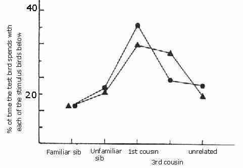
This graph after Figure 2 in Bateson (1982) shows the mean percentage time spent by adult Japanese quail near members of the opposite sex that were either familiar siblings, novel siblings, novel first cousins, novel third cousins, or novel unrelated birds. The chance level was 20%. Triangles are averages for 22 males, and circles means for 13 females. From Patrick Bateson Mate Choice (Cambridge University Press Cambridge 1983)
This does not appear to be the case with humans in my experience.  It would appear that humans are not honest with our feelings.  There is also the reasoning that when an individual or a population is doomed selection has no way to offer survival clues.  In fact, since a population doomed by excessive outbreeding is a threat to the whole species, selection should try to eliminate that rogue population as fast as possible.  One way to do that is to cancel the kin attraction.  Of course in order for speciation effects to eliminate a population, two thousand generations must pass.  The mechanism limiting fertility under conditions of outbreeding works much faster.  But as we said, although nature takes the long view – eliminating a population thousands of generations before it can wreak its havoc – nature cannot see the big picture.  In our case essentially every part of the species is involved in the oubreeding spree.  Selection is plucking us out everywhere at the local level oblivious to the fact that this is global.  Humans, fixated on the short term, are not concerned.
Another example: (Playing Kissy with the relatives SCIENCE vol. 342 no. 6163 December 6, 2013 page 1147 reviewing Nat. Struct. Mol. Biol. 10.1038/nsmb.2699 (2013) shows that bacteria also have a preference for mating with kin when, indeed, they do mate.   
This should be the end of the analysis.  I have argued starting at first principles that any complex life form population must have an intrinsic limiting mechanism.  I have presented evidence that such a mechanism is present and at work among humans and other animals.  The evidence comes from multiple independent sources.  I cannot think of any scientific principle that had so much evidence in its favor that did not at least stir controversy.  Surely it is time to pass on the torch.  Somebody ought to run down the mechanism so that if the impending doom that seems to be threatening us can be addressed and if possible a cure found. 
But this has not happened.  So I have begun to work out the mechanism.  The first step was to do an experiment, which I did with a colleague.  This was published in African Entomology.  M.L. Herbert & M.G. Lewis Fluctuation of fertility with number in a real insect population and a virtual population African Entomology 21(1): 119–125 (2013). 
Since we are talking about changes in birth rate the broad topic is “infertility.”  Infertility is broken down in medicine into the headings pre-zygotic and post-zygotic.  Things that prevent a sperm from combining with an egg to become a zygote are pre-zygotic while things that prevent the zygote to develop into a fertile adult are post-zygotic.  I have a small problem with the distinction.  Reproduction is cyclic.  An event that is post-zygotic with respect one cycle must surely be pre-zygotic with respect to the subsequent cycle; the distinction seems a bit arbitrary.  But I find that once you sit down to write a computer program to model infertility as a consequence of insufficient kinship the distinction is anything but arbitrary.  You simply must be explicit about what kind of infertility you are interested in.  It’s straightforward enough to build a model that has both kinds of mechanism running at the same time, but I have not figured out a way to leave the question unanswered. 
Our experimental model was much like the Calhoun study of mice.  We prepared a sixteen fruit fly lines, each descended from sixteen different commercially available lines, which had been added in a different sequence for each of our experimental lines, thus assuring we had ample genetic diversity at the outset and there were no specific incompatible gene pairs that we could detect.  We then released the flies into a large cage prepared to be as commodious as we could easily build and attend to.  Then we detected two windows of specific size and counted the number of flies in the windows daily for two years as a way of following population size and inferring fertility. 

Fig. 1. Raw counts pooling both windows for two weeks. The vertical axis is the accumulated counts. The horizontal axis is time. Counts started on 7 July 2008 and continued to 11 July 2010.

It soon became clear that the flies tended to spend the night sleeping on their food.  There were many dead flies to be found in the food as well as elsewhere in the cage.  Accordingly on two occasions an ordinary plate with food was placed in the cage for a few days.  The plates were inspected at all hours during the night, and it was found that although many flies took advantage of the supplemental feeding, at no time did they come close to occupying all the available space so if the population was being limited because the flies were tramping each other into the culture medium, it was not because they had no choice.  As with the Calhoun experiment there was always space as well as food for more.

One can tell at a glance that the pattern here is neither the single peak followed by extinction that Calhoun’s data and the plague show nor the double peak with extinction that Diamond’s data and the plague data show.  There is a mechanism governing the population, but it is not the same as with mice and people.

I prepared a computer program that modeled pre-zygotic and post-zygotic infertility and the combination.  Of course it was necessary to tweak the parameters to get significant restriction of the virtual population without extinction.  This is what I found with a pure post-zygotic program.

Fig. 2. A single run of a computer program modeling a population affected by post-zygotic infertility increasing with decreasing consanguinity and increasing population size.

The experimental study shows four peaks, decreasing in height each cycle, and four troughs, also decreasing each study.  The model shows three decreasing peaks with three decreasing troughs.  After the cycles both the model and the experimental population become less predictable.  The experimental demonstration is more elegant than the model, which I think is not the usual case.  That is not to say even this degree of fidelity to the real world happens each computer run.  Because of limitations of RAM (random access memory) available the computer simulation is pestered with stochastic chatter. 

In contrast, here is a computer run in which the mechanism is pure pre-zygotic.

Fig. 3. A single run of a computer program modeling a population affected by pre-zygotic infertility increasing with decreasing consanguinity and increasing population size.

Don’t worry, it’s not that bad, not quite.  What we see is a virtual birth rate that declines, seems to be stabilizing and then abruptly goes to zero.  That brings to mind the UN study showing the birth rate in developed countries falling and then leveling off.  Were humans affected by a pure pre-zygotic mechanism we might taka alarm and wonder whether our own birth rate might show a similar abrupt failure.  The line is also hauntingly reminiscent of the Calhoun study in which population size was still rising on the day of the last live birth.

In contradistinction from the pure post-zygotic mechanism, the results are quite robust.  If the maximum population is kept low enough then the population will continue.  If the maximum population is allowed to rise even higher, then the end comes sooner.  However, this pattern does not and in my hands cannot account for the double peak pattern seen in the Diamond and the mouse plague data and the historical data.  This cannot be the mechanism we are living with.  However if, with suitable tweaking of parameters, you run both pre-zygotic and post-zygotic at the same time you can get this.

Fig. 4. A single run of a computer program modeling a population affected by pre-zygotic and post-zygotic infertility increasing with decreasing consanguinity and increasing population size.

Now we have the statistical noise introduced by both programs at the same time.  The pattern is almost invisible, but it is a least arguable that we have two peaks, the second one terminal.  The first peak is much higher this time, because instead of the genetic diversity that appears to be the requirement for the double peak in history and in nature, our initial population was a virtual cone, so of course fertility was maximal to begin with. 

So what appears to be going on in real life is that when the population gets too big the post-zygotic mechanism starts to have an effect and induces the oscillation that is its hallmark.  Then on the second cycle, in mammals, the pre-zygotic mechanism, which one must suppose takes a bit longer to be activated, cuts in and finishes the job.

With the help of a little hand waving it is possible to suggest that this is happening to people now.  Sperm counts are falling.  I attended a meeting of the American Society for Reproductive Medicine.  One of the speakers was a woman from the UN who announced that because sperm counts were going down all over the world the normal range was being lowered.  I was rather surprised that the other doctors sat there and heard the news without batting an eye.  It turned out that this had happened before. 

I have seen a fair amount of controversy about what sperm count means and how to do it.  Sperm vary not only in number but in concentration, in the rate of deformity of sperm and in their motility; I suppose they differ in average lifespan, too, although I have not seen that mentioned.  Still, sperm count must be real and must be significant or she would not have come with the news.

Nowadays many couples working at establishing a pregnancy turn to direct sperm injection.  Instead of the old fashioned way and the pretty old fashioned way of putting the egg and sperm into a dish, a likely egg is chosen as is a likely sperm and the sperm is placed into egg with an instrument by main force.  The process is repeated.  The zygotes are cultured and after a time one or more of the best looking ones are implanted in the womb.  Frequently the process works just fine.

Since the characteristics of the sperm are vital to its function both in vivo and in vitro it is understandable that some debate has ensued.  I have heard a rumor that the results of in vitro fertilization are not above reproach, but that is not of great consequence if the alternative is no pregnancy at all.

The interesting thing here for us is that any difficulty with sperm must be post-zygotic.  A different man would make different sperm.  Since injecting sperm often is needed and often succeeds, I think there is an excellent case for there being widespread post-zygotic infertility.  I have also heard rumors that penis size is decreasing and rate of deformity increasing, but sperm count is enough to say there is evidence for post-zygotic infertility on a global scale, just as we would expect. 

If you google “gapminder.com” you should find “Gapminder: Unveiling the beauty of statistics for a fact based ...”  Click that.  Click “load gapminder world.”  Give it a moment.  A graph comes up for a particular year with a number of circles representing countries; bigger circle means bigger population.  There is an arrowhead indicating a dropdown menu at the bottom.  Click it and then choose “Children per woman” at the top.  Give it a bit to load.  Now go to the left hand side and open the dropdown.  Second from the bottom is “Population,” which opens another dropdown.  The bottom of that menu is “Age at first marriage (women).”  Click it.  Drag the date slider down at the very bottom all the way over to 1800.  Click “Play.”  For the first 150 years you will see an overall tendency for birth rates to decline (move to the left) but not much action in age at first marriage.  Then for the next thirty years there is a decided decline in birth rate.  After 1980 there is a spectacular rise in age at first marriage.  Once birth rates fall below replacement, they stabilize, as we have seen before.  But by and large starting at that time the women wait longer to marry.

Their biological clocks are slowing down.  You remember the biological clock.  It used to be said in hushed tones.  When a woman’s body said, “Time to do it,” she was going to get pregnant come hell or high water.  And now they are stopping.  All right, is this pre-zygotic or post-zygotic?  I won’t swear to it, but it seems to me we are looking at sperm-doesn’t-find-egg rather than egg-doesn’t-look-for-sperm.  I’m not sure.  And I am the one who wrote the program.  Still, it does seem that there are two mechanisms at work.  The dynamic graph is most eloquent on that one. 

Here is the line for Sweden in recent years.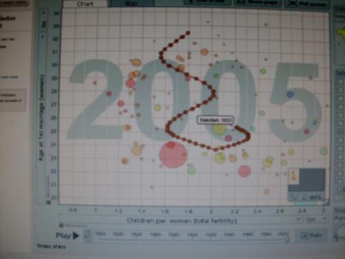
There is more than statistical evidence for the two mechanisms.  A team raised some plants in earth with chemicals that stripped methyl groups from the plant DNA.  I am surprised that the plants mangaged at all.  Methyl groups (If you take a carbon with four hydrogens attached, that’s methane.  If you strip a hydrogen off and attach the free bond to another chemical, then you have added a methyl group to that chemical) on DNA are a way of regulating the function of the DNA.  But the plants managed.

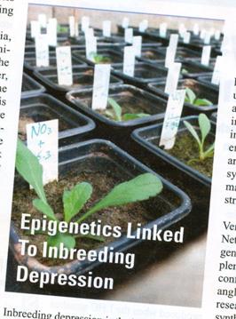
 (Elizabeth Pennisi Epigenetics Linked to Inbreeding Depression SCIENCE vol. 333 no. 6049 September 16, 2011 page 1563 reviewing work by a team led by Philippine Vergeer, Hugens Building, Room HG 01.132, Radboud University Nijmegen, Molecular Ecology, Heyendaalseweg 135, 6525 AJ Nijmegen, The Netherlands p.vergeer@science.ru.nl )  What they found was that if plants that had been subjected to inbreeding to the point of inbreeding depression were sprouted in an environment with a demethylating agent deleterious effect of the inbreeding was completely removed.  As long as I have taken an interest in such things I have been told that inbreeding is undesirable because you get two copies of a gene and that’s b-a-a-a-a-d.  And now it turns out to have nothing to do with genes at all.  It’s all epigenetic (has to do with control of genes). 
The treated plants were as healthy, and one must conclude as fertile, as plants innocent of all inbreeding, maybe more fertile.  Quick on the scent, we ask now whether the infertility of inbreeding depression is pre-zygotic or post-zygotic.  Of course it makes intuitive sense that it is post-zygotic, but we can check that.  This summarizes a series of computer runs using a pre-zygotic mechanism with varying maximum population size and all other parameters held constant.

Computer simulation of a population restricted by pre-zygotic outbreeding depression.  Average over 10 repeats.  Number of offspring in generation 1,000 is on the vertical axis, size of population is on the horizontal axis. 
There’s no inbreeding depression there.  The highest fertility is at the smallest population.  On the other hand here is a similar series with a post-zygotic mechanism. 


Computer simulation of a population restricted by post-zygotic outbreeding depression.  Average over 10 repeats.  Number of offspring in generation 1,000 is on the vertical axis, size of population is on the horizontal axis. 
Yes, it’s a dirty graph.  It bounces around because average offspring is total offspring divided by population size.  If you have an even number of offspring in your population and add one more, then your denominator rises but the new member of the virtual population does not find a mate and the numerator is unchanged.  Ignoring that, and the fact that the very smallest population is an outlier, yes we do have inbreeding depression.  So we know that, at least in plants, inbreeding depression is not genetic but epigenetic and that mechanism is post zygotic.  
I feel rather smug about that.  It’s a lot to learn from a few potted plants and from tapping a few keys.  Before I accept that inbreeding and outbreeding depression in fruit flies and humans is not epigenetic with DNA methylation as the cause, somebody is going to have to produce some very impressive evidence.  I suppose you have noticed that the right hand part of the curve is the Sibly curve all over.  The whole curve is the Iceland and Danish data. 

So what about a pre-zygotic process?

Some people did a study of deermouse sperm bunching together to form a sort of flying wedge that lets them swim faster and possibly reach an ovum before other sperm. 
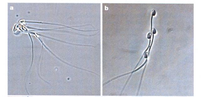 Pictures from Competition Drives Cooperation Among Closely Related Sperm of Deer Mice, Heidi S. Fisher and Hopi E. Hoekstra, NATURE vol. 463. no. 7282 February 11, 2010 page 801. 

They will not do this with unrelated sperm.  If a sperm can recognize related sperm it is reasonable to suspect (although the study begs to be done) that sperm can recognize related ova.  If so, the failure to do so would be a pre-zygotic depression of fertility. 

Before leaving the computer simulations altogether, I promised that I would return to the pattern of exponential growth in black footed ferrets and humans and how it departed from pure exponential. 
Here is another example of fertility in a virtual population limited by a post-zygotic process followed over time:
 
The curve is truncated because the program can only deal with a finite number of members of the population and their potential offspring, but as you see the population can oscillate with a characteristic shape.  I’ve lost my notes, but when I looked at the nearly exponential rise of each curve it departed from pure exponent in the same fashion as ferrets and folks. 
We are about done.  Let me insert a cautionary note. 
Some people counted voles in Europe and followed their population size.  Have a look and see whether they look like our data on fruit flies:

Thomas Cornulier et al. Europe-Wide Dampening of Population Cycles in Keystone Herbivores SCIENCE vol. 340 no. 6128 April 5, 2013.  Only part of the data shown.
Sorry about the resolution, but bear with me and confine your attention to the dark line in the graph in the top left hand corner.  The dark line is annual spring counts of voles taken in Sweden from 1970 to 2010.  The cycles occur at a rate of three per ten year interval.  With our flies we reckoned the time of the cycle from peak to peak was about 5 months or five generations of flies the way we had it set up.  If we apply that to three cycles in ten years we get about a 40 month cycle.  At five generations per cycle that would suggest that voles have about an 8 month generation time.  You can decide whether this is reasonable.  If you look over the mouse data, you can decide whether they go through cycles five generations long. 
The problem to me is that these curves look like the curves for the fruit flies.  And voles, like people and mice, are mammals.  They should exhibit the Calhoun pattern or the Diamond pattern, I should think.  At least the fact that the fruit flies do not encourages me to think that the flies lack a post-zygotic mechanism.  Perhaps the local populations never rise to the point where the pre-zygotic mechanism is activated.  But if that argument holds, why should it not hold for the flies?  So I am left not totally sure.  But as for kinship and fertility being related, it does seem undeniable.  The possibility must be entertained that this is an existential threat to humanity. 

There have been 143 visitors over the past month.
Home page.