This poster was presented at the international genetics convention in Brisbane in 2006.
Effect of Size on Virtual Population Growth

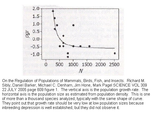
Sibly et al estimated the relationship between a population's size and its growth rate for 1,780 time series of mammals, birds, fish, and insects. Growth rates are high at low population densities but, contrary to previous predictions, decline rapidly with increasing population size and then flatten out, for all four taxa. This produces a strongly concave relationship between a population's growth rate and its size.  The fact that the curve is defined by only three values (vertical and horizontal position and degree of curvature) suggests a simple scientific law lying at the very heart of evolution and, we suggest, genetics.  We undertook to duplicate the curve with one of two programs we had available that could simulate a population, specify details of its genetic behavior and follow it over generations. 

                     A                                            B

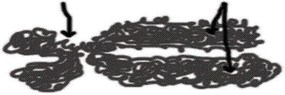
Recent work on the speciation of Anopheles mosquitoes (Microarrays and Species Origins.  Roger Butlin and Cally Roper.  NATURE 437: 199-201 SEPTEMBER 2005) has found that “speciation genes,” which appear to be causing speciation, are located near the centromeres (A) of the chromosomes, a region that does not undergo crossing over. 

Of two programs we had, one modeled genes that assorted independently or were loosely linked, which would be like genes located at a distance from the centromere (B) or on different chromosomes.  The other program had all genes rigidly bound to one pair of chromosomes.  This proved to be the program that was able to reproduce the concave curve described by Sibly et al.

Spread Sheet of Growth Rate of Different Population Sizes

Graph of Growth Rate against Population Size

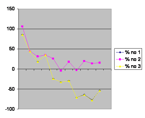
Simply assigning 0 population to the extinct line is “% no 1” on the graph.  “% no 2,” dropping the populations that go extinct from consideration, underestimates growth reduction, but is the approach used by the authors.  They, too, observed that local populations go extinct in the wild all the time.  % no 3 takes the maximum population size, divided by the number of generations it took to go extinct, and winding up with a number lost per generation, subtracting that from the sum of the offspring in the populations that survived.  This approach is still not perfect, but does give us a line, % no 3, which is essentially the same as % no 1.  Compare with page I.

Where Evolution Places a Genome

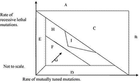
The model accounts for observations, but there are more variables in the model than in reality.  There must be some simplifying mechanism.  That mechanism is evolution.  In the chart A, B, and C are forbidden because the excessive mutation rate would produce extinction.  E is not plausible.  D we doubt to be possible.  F is possible for a finite time, but evolution will increase complexity in the direction of arrow G, until complexity is maximized in H.  This is an intrinsic limit to evolution.  (In Search of the Limits of Evolution.  Fyodor A. Kondrashov  NATURE GENETICS: 17: 9 January, 2005) .  A subset of H, I, will have the properties we have shown.  The fact that evolution must stop in H explains punctuated equilibrium.  Evolution starts anew when a form is returned to F because of a favorable change that permits survival with less performance, such as domestication or monogamy. Driving all forms into I reduces the variability that can be observed.

Home page.